Sections
The product, shown in the figure below, is a compilation of eight different GCMs, using CMIP5 and RCP 8.5. A study was also conducted looking at the relative variation of GCM predictions versus RCP scenarios versus ET estimations and we found that of the three, the differences among RCP scenarios were the smallest.
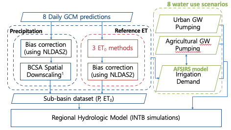
A new downscaling method was developed, seen in the figure below, by Florida Water and Climate Alliance with the eight GCM projections. First, there was bias correction then downscaling, both the precipitation and reference ET. We found that univariate bias correction was much more efficient computationally.
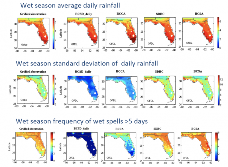
Bias statistical downscaling was used because we had eight GCMs. There were not eight dynamically downscaled GCMs for the scale that was needed so we decided to use a statistical downscaling method, and ended up developing a new one because when we looked at the existing national products, they did not represent the spatial-temporal rainfall characteristics in Florida very well. The choice of downscaling method you use in Florida matters, and it depends on what you intend to do with that data. The method developed is called the Bias Correction Stochastic Analog (BSCA) Downscaling Technique.
The results of the comparison are presented in the figure below. On the left-hand side you can see the gridded observations of daily rainfall characteristics in Florida. These four columns represent the four different ways the data was downscaled. The final column is the Bias Corrected Statistic Analog (BCSA) that we developed. Some of the other versions do not do a good job of reproducing daily rainfall variations. Here though, you can see BCSA does do a good job reproducing the daily rainfall variations throughout the year. The first two methods also do not do a great job of capturing the variability between wet seasons and dry spells.
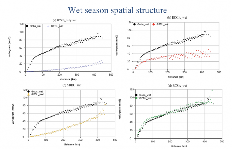
Another important aspect driving Tampa Bay’s integrated hydrologic model was the spatial variability of the rainfall. The four plots in the next figure measure how variable this rainfall was over space with further distances. The top lines represent observations.
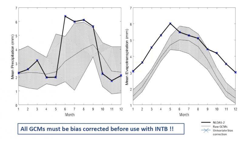
In the figure below, the graphs show the eight GCMs over the Tampa Bay region and the whole state of Florida. The gray envelope is the variation across the eight GCMs, and these are mean values each month. The data must be bias-corrected in order to reproduce the respective hydrology. Once that is complete, the GCM data perfectly matches the historical data.
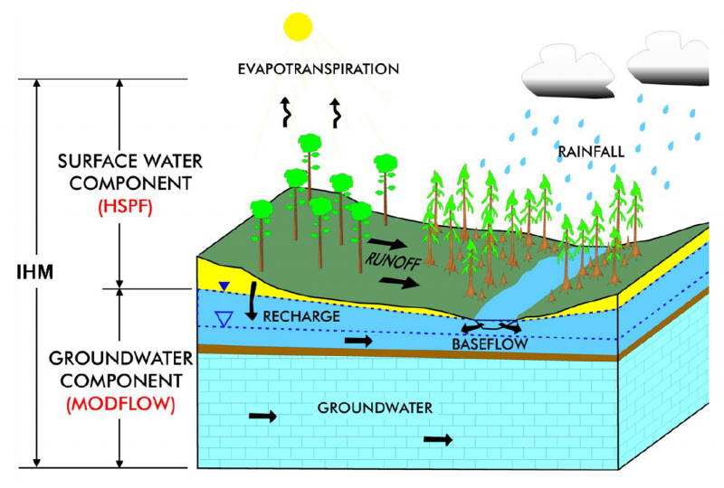
The hydrologic model we are using is a couple of HSPF mod-flow models that have been calibrated to local rainfall weather station data. The figure below is an example of an Integrated Hydrologic Model (HM).
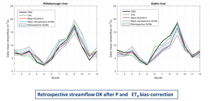
These next graphs show data for the Hillsboro and Alafia Rivers, which are the two that the Tampa Bay Watershed draws from for water supply. These are the mean monthly observations over the retrospective period, which was the calibration period (I believe) 1982 to 2006. The black line shows the observations. The green line is the model that was calibrated with the local weather station data. The red line is the model driven by NLDAS-2 data, which is the national gridded product of weather data over the entire continent. The blue envelope is the eight GCMs to predict retrospective hydrology.
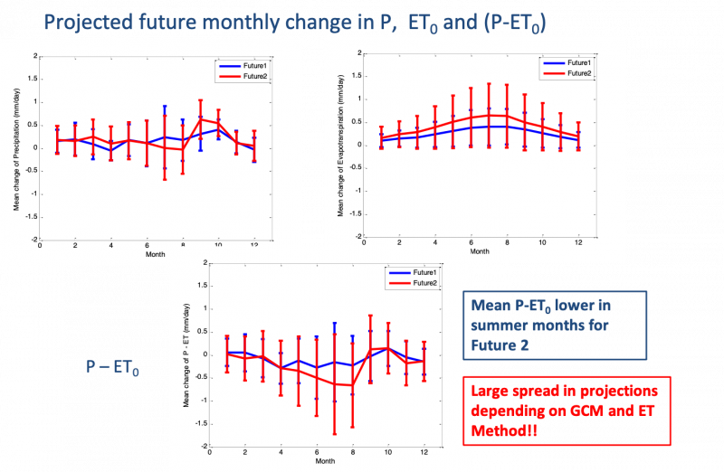
The image below shows the projected future changes in monthly precipitation, potential evapotranspiration, and water availability not put through the hydrologic model yet. These results are for the entire state of Florida. The blue line is Future 1, which is 2030 to 2060. The red line is Future 2, which is 2070 to 2100. Both models are predicting slightly higher monthly mean precipitation. You can see there is quite a bit of variability between the GCMs and ET method.
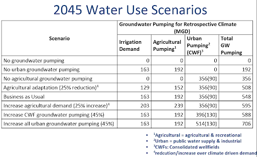
Tampa Bay Water’s Urban demand is projected to be about 280 MGD (million gallons per day) in 2045, assuming active water conservation. Climate-driven agricultural irrigation water demand is estimated by the AFSIRS model using GCM future projections. Land use change is not considered. Increases in demand are assumed to be the result of intensification on existing lands.
These eight water supply scenarios were created to look at the relative uncertainties of climate projections versus water use projections on water use hydrology. The scenarios range from no groundwater pumping for agricultural or regional water usage to relaxing the current groundwater pumping permitting requirements by 45%.
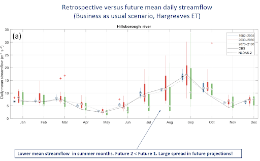
This plot in the figure below shows the business as usual scenario, using the Hargreaves estimation method, looking at projections on daily streamflow in the Hillsborough River. The blue is retrospective, the red is Future 1, green is Future 2, and black is retrospective observed and the calibrated model. There is a substantial range in variability. There is also wide uncertainty due to the fact that there are only GCMs in this particular plot.
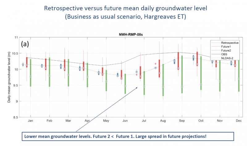
This plot in the next figure is for a particular groundwater monitoring well located near a wetland with regulations to limit groundwater pumping to protect the wetland integrity. Again, there is a similar projection that groundwater levels are dropping from retrospective to Future 1 to Future 2, especially during the summer. There is substantial uncertainty across the eight GCMs.
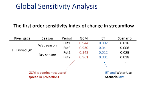
A Global Sensitivity Analysis was projected across the GCMs, ET method, and water use scenarios to understand and identify the biggest drivers of uncertainty. When looking at streamflow projections, the GCMs are driving the range in the box and whisker plot. The ET method and water use scenarios are much smaller. The results are in the table below.
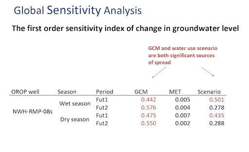
In this second analysis (results below), the GCM and water use scenarios are more equivalent. This is largely because the groundwater prediction is more local, located near a wetland, and is influenced by urban pumping. Comparatively, the streamflow is an integrated quantity over the entire watershed.
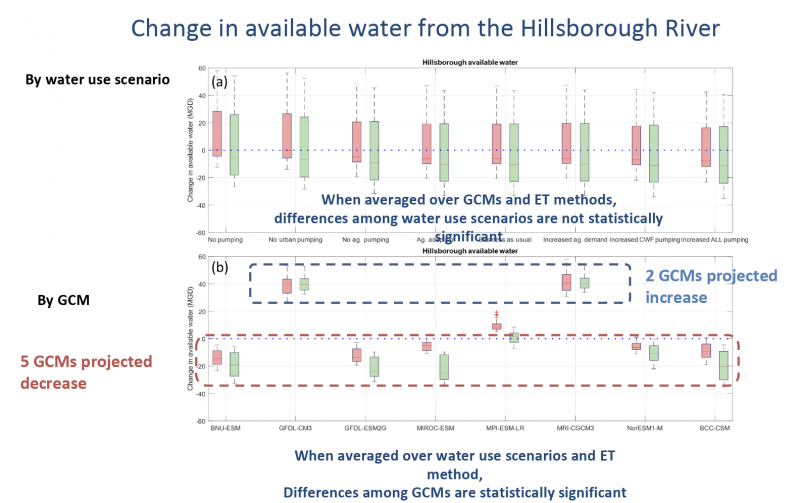
Tampa Bay Water uses waterflow from the Hillsborough River. It is restricted to a certain volume depending on the time of year. We were looking at how the available water from the Hillsborough River changes in our projected future. This next figure shows the change in available water from the Hillsborough River and water use scenarios. The left shows no groundwater pumping and the right is increased urban and agricultural pumping due to the variation in GCMs and ET estimation methods. The differences across GCMs are significant, and the differences between water use scenarios and ET methods are relatively smaller.
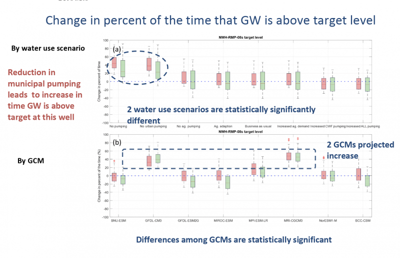
The figure below shows a relatively same idea for groundwater. Again, groundwater influences are more local. For example, by halting or decreasing groundwater pumping, you could increase the time the groundwater is above the target level.
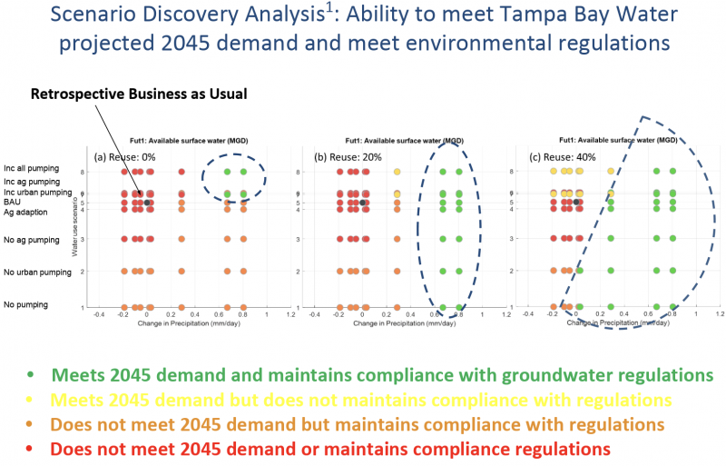
Next, we wanted to look at these scenarios to uncover our vulnerability. We did a scenario discovery analysis to look at all of these different scenarios and projections to determine which ones would be able to meet both Tampa Bay Water’s 2045 demand and environmental regulations. The most important distinguisher between the GCMs was the projected change in precipitation. In a future where there was no reuse of wastewater to supply irrigation or more direct potable water reuse, and no increase in desalination capacity, there were only four scenarios that both met the 2045 demand and maintained compliance with existing groundwater regulations. They were the two very wet GCMs in which groundwater regulations were more relaxed so more water could be pumped, but could also happen due to increased rainfall. If we increased reuse by 20 or 40%, you can see increased possible scenarios in the figure below. However, these are the water use scenarios that completely convert the urban water use to surface water.

