Sections
How has the climate in the United States changed from the beginning of the last century to 2015?
- Global temperatures have increased since the middle of the 20th century.
- There is an observed overall warming trend over much of the U.S. during this period.
- Precipitation is more challenging to assess, is complex, and shows much seasonal variability.
Your assessment toolbox will, most likely, contain some sort of climate projection. What is a projection and how does it differ from a climate prediction?
A projection is:
- A plausible future condition, one that falls within the laws of physics.
- Often based on the results of a climate model.
- Not assigned a probability.
- Often called a scenario.
A prediction is:
- Also known as a forecast.
- A most-likely expectation.
- An outcome associated with a probability. These can be precise statements about the future, such as:
- "There is a 70 percent chance of rain tomorrow,” or
- “Global mean temperatures will rise 4–11ºF by 2100 over the mean for 1960–1990.”
There are a wide variety of climate models, with varying degrees of confidence depending on the time scale, the spatial scale, and the variables involved in the model. It’s important to have a sense of how confident you can be in the results of a specific model so that you can select the best model for your needs. The table below lists some of the elements that determine the confidence level for models projecting future climate change.
| More confidence | Less confidence |
|---|---|
| Global and continental-scale projections | Regional and local projections |
| Averages | Extremes |
| Directions of change | Magnitude of change |
| Temperature is the dominant process | Physical processes other than temperature are dominant |
The graphic depicts the continuum of certainty related to climate change models.
Evaluating potential future climate conditions is difficult because non-climate factors are difficult to anticipate. Human activity and future emissions, the physical response of the climate system (e.g., climate sensitivity and regional patterns and timing of change), natural climate variability, and interpreting climate models (e.g., through downscaling or hydrologic modeling) are all very difficult areas of knowledge, investigation, and, by extension, prediction. The following sections explore each of the key sources in greater detail.
There are important uncertainties involved with predicting future greenhouse gas (GHG) emissions (carbon dioxide [CO2], methane [CH4], etc.) Economic activity, technology, policies, and many other factors also impact GHG levels. The sources and effects of increased aerosol levels (such as soot and dust) in the atmosphere are another subject of intense scientific inquiry. Finally, land use practices can have dramatic effects at the local and regional scale.
Because emissions are difficult to predict, the Intergovernmental Panel on Climate Change (IPCC) uses Representative Concentration Pathways (RCPs) conditions to develop future climate scenarios. In a nutshell, RCPs identify a total amount of additional energy that would be trapped by greenhouse gases, expressed in units of radiative forcing in watts per square meter (W/m²). More greenhouse gases in the atmosphere equals more radiative forcing, which in turn results in an increase in global temperatures.
Earth’s atmosphere currently contains about 2.8 W/m2 of GHG-forced radiation above pre-industrial levels. Doubling of CO2 concentrations over pre-industrial levels would trap a total of 4.5 W/m2.
RCPs are scenarios and don’t have likelihoods assigned to them, so we don’t yet know which one to plan for.
The table identifies the various RCP scenarios currently in use. The number value of each represents the amount of radiative forcing each scenario is projected to produce in W/m2. The Climate Model Intercomparison Projects (CMIP) are adding RCP 7.0, which may be the most likely—we just don’t know.
| Baseline scenarios | |
|---|---|
| RCP 8.5 |
|
| RCP 6.0 |
|
| Stabilization scenarios | |
| RCP 4.5 |
|
| RCP 2.6 |
|
| RCP 1.9 |
|
How do you, as a practitioner, use these models in assessing vulnerability of your water resource? Which scenario is the best fit for you, your customers, and your region, and how much risk do you want to accept when planning for the future?
The answers to these questions guides which scenario you will select.
With a doubling of global CO2 amounts, the temperature of Earth’s atmosphere is projected to rise between 3.6ºF (2°C) and 8ºF (4.5ºC). It is very unlikely that it will be below 1.8ºF (1°C) or above 11ºF (6ºC). Be aware of the inherent uncertainty in these projections and be prepared for changes in these values as modeling and analysis techniques evolve.
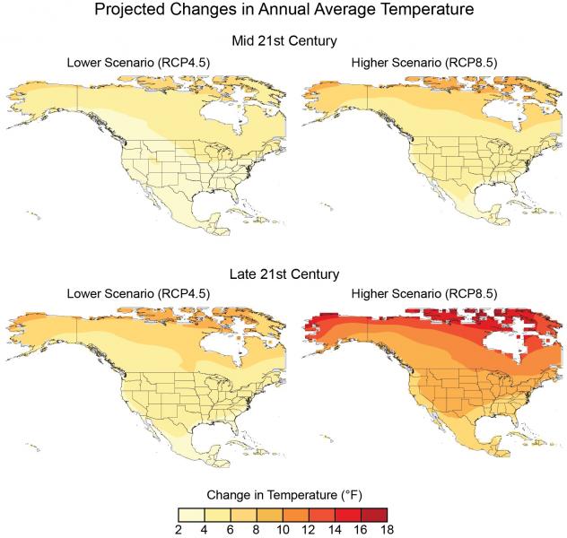
The maps below show the projected relative changes in temperatures in North America under the 4.5 and 8.5 RCP scenarios. Note that the colors reflect average temperature change, not actual temperatures. For example, under scenario 8.5 in the Late 21st Century, the Arctic will not be hotter than Florida; it will just have experienced a greater change in annual average temperatures.
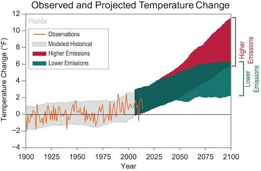
In the graph, both scenarios look very similar for the next few decades, which demonstrates why it’s so difficult to know which scenario we’re currently experiencing. The data can, however, help you decide which RCP scenario to use in your plan. If you are looking to find solutions for the next couple of decades, then a lower emission RCP may suit your needs. Planning for many decades would require one based on higher emissions.
Note the percentage change in seasonal precipitation projected across the continent under RCP 8.5 in the maps below.
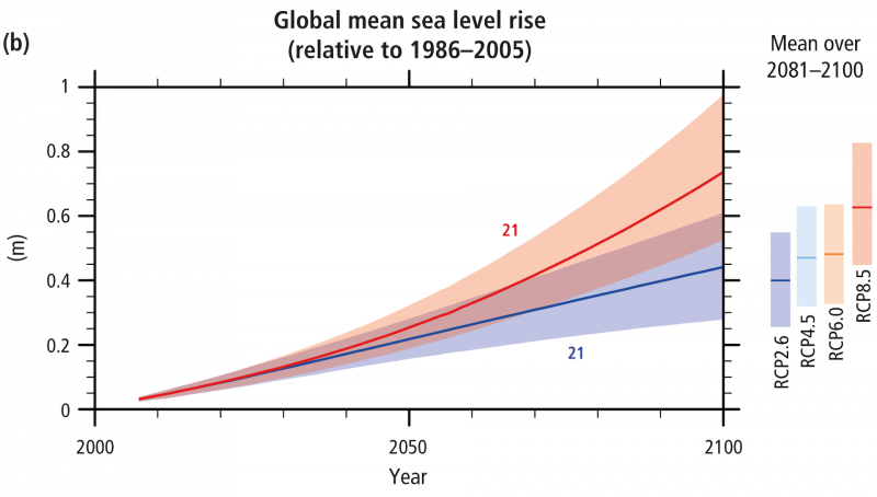
Projected global sea level under various RCP scenarios are shown in the graph at right. As with all projections, uncertainty exists in the models.
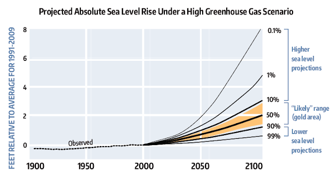
Finally, the graph below takes sea level rise projections one step further and applies probability to the IPCC data. In this study, there was a 90 percent probability that the IPCC scenario was accurate, a 10 percent chance that sea level rise would be greater than three feet, and a 1 percent chance that it will be greater than 4.5 feet.
Climate variability has—and always will—exist. Note that the overall climate trend is often masked by “noise,” a statistical term describing variability in a dataset. Noise is what leads people to make comments such as, “How about this global warming? It’s 30°F here in Florida in February!” Cold days will happen in Florida, but the overall trend is gradual warming.
Multi-year and multi-decadal events more accurately represent long-term variability and data. Some examples include:
- The El Niño Southern Oscillation (ENSO)
- The Atlantic Multi-decadal Oscillation (AMO)
- The Pacific Decadal Oscillation (PDO)
How these will be affected by—and will affect—climate change is not clear. Natural variability matters, but it doesn’t show a long-term trend. Human activity and the consequent rise in emissions does show a long-term trend.
Climate variability may be changing, too. We’re seeing more extremes. For example, one year may be very wet and the next very dry, and we’re seeing more “whiplash” as the climate shifts from one extreme to the other rapidly.
Models are the only way to project change in climate resulting from human activities. There is no analog for human-induced warming. We’re unable to carry out deliberate controlled experiments—there’s only one Earth.
The system is very complex, so climate models are our best source of information...but they aren’t infallible. Models are improving in terms of resolution and the processes they simulate. Model agreement is not a forecast.
Climate models are used to project how human factors affect Earth’s climate. We rely on models to test our different questions and assumptions. Models are not crystal balls, but as simplifications of complex realities they are the best sources of information we have. Models are improving in regards to computer simulation and the resolution and the processes they simulate.
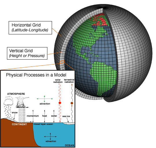
Global Climate Models (GCMs) are also known as General Circulation Models or Earth System Models. They model the entire Earth system, including the atmosphere, oceans, land and vegetation, and the cryosphere (Earth’s ice).
They divide the system into grid boxes. Typical grid boxes in GCMs are about 2 to 3 degrees (about 120 to 180 miles across), although some are higher resolution. Each box assumes uniform conditions. How well a model simulates climate processes matters much more than its resolution.
Models underlie all the projections we use for climate change. Global Climate Models have relatively low resolution. GCMs give a uniform projection for each grid box and cannot account for sub-grid scale processes (for example, convective thunderstorms aren’t shown on GCMs). GCMs are also particularly problematic along coasts and in mountains. Resolution is improving because of computing power. Capabilities are improving as well, and models can display many processes that were previously unavailable in a GCM.
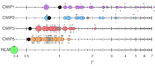
- The figure above shows data from different models. The green circle designates a perfectly accurate model. The further to the right a circle is, the less accurate it is. The black circles represent averages.
- With each generation of models, the simulation of the current climate improves.
There are two kinds of model averages, known as ensembles. The first averages the results of many different global models, and the second averages multiple runs from the same model under different initial conditions.
The average of climate models’ simulations of current climate is generally closer to observed climate than any individual model. Averages don’t show range, which is important (especially when looking at climate variability), but averages can be used as a scenario.
A good rule-of-thumb is to seek the support of experts if your work involves use of models.
It is possible to take a model with course resolution and focus in on a smaller area using a process called “downscaling.” We downscale because we want information at a higher resolution. Higher resolution is not necessarily more accurate, but it can provide more insight at a regional level.
The key question should be how downscaling improves the results:
- Do the results make physical sense?
- Do we better understand the direction of change at a high resolution?
- Do they project how change varies within the GCM grid box?
- Does downscaling provide more accuracy or just precision?
- Does it give us insight into sub-grid scale processes?

